Urban Drone Pathfinding

Sep 10, 2024

#Projects

Read time: 41 minutes

Introduction

The goal of this project is to localize a drone as it navigates through a city. I am given some data about the drone's movements and its surroundings, and my task is to estimate the exact path the drone takes as it moves through the city. The city map consists of roads and obstacles, and I need to determine the drone's path based on the provided data.

I chose to write Python code for this drone localization project instead of using Monte Carlo methods from the start. My goal was to improve my coding skills and deeply understand how to solve the problem through coding. By doing this, I gained insights into the problem and explored alternative approaches. The next step is to apply Monte Carlo localization to see if it improves the accuracy of the drone’s pathfinding.

Problem Explanation

I have several key pieces of information that help me understand the problem:

City Map

The map is provided in two formats:

- A text file (map_stadi.txt), where:
- The value 0 represents roads where the drone can move.
- The value 1 represents obstacles that the drone cannot pass through (such as buildings or walls).

- A background image (map_stadi_bg.png), which visually represents the layout of the city (roads and obstacles).

Drone's Movement Data

I am given a file (drone_path.csv) that contains odometry data. Odometry data is a measure of how the drone is moving, specifically providing two coordinates for each step:

- x_odometry: How much the drone has moved in the x-direction.

- y_odometry: How much the drone has moved in the y-direction.

However, these movements are noisy, following a normal distribution with a variance of 4.4. In reality, the drone's movement might be slightly off from what the data reports.

Lidar Measurements

The drone is also equipped with a Lidar sensor, which works by sending out laser beams and measuring how far away objects are. This data is provided in a file (drone_log.jsonl) and contains 36 measurements for each step the drone takes. These measurements are spread out over 360 degrees, with each beam covering a 10-degree angle.

Like the odometry data, the Lidar measurements are also noisy and follow a normal distribution, with a variance of 0.1.

Objective

Using the data provided, I will estimate the drone's true path, ensuring that the drone does not cross obstacles and stays on the road. The final output will be a file that lists the coordinates of the drone's actual path.

Let's start!

We need to import the necessary libraries for data processing, visualization, 3D handling, and mathematical operations.

import matplotlib.pyplot as plt
from math import sqrt
import open3d as o3d
import pandas as pd
import numpy as np
import json
import csv
import math

Now I need to load the map and sensor data from the provided files. Then, I define constants like noise variances and the angular resolution for Lidar measurements:

# Load map data from TXT file
map_txt_file = 'map_stadi.txt'
with open(map_txt_file, 'r') as file:
    map_lines = file.readlines()

map_data = [[int(value) for value in line.strip()] for line in map_lines]
omap = np.array(map_data)
omap = np.flipud(omap)

# Load sensor data
with open('drone_log.jsonl', 'r') as file:
    sensor_data = [json.loads(line) for line in file]

# Define constants
NOISE_VARIANCE_ODOMETRY = 4.4
NOISE_VARIANCE_LIDAR = 0.1
ANGULAR_RESOLUTION = 10  # in degrees

Now let's define helper functions to simulate how a Lidar sensor measures distances to nearby obstacles. The measure_distance function calculates the distance in a specific direction until it hits an obstacle or reaches a boundary, while the observation_model uses this function to gather distance measurements in all directions (0 to 360 degrees).

# omap = occupation map
# x0,y0 = position of the lidar
# vx,vy = single pixel unit vector to some direction we want to measure the distance
# max_steps = maximum range of the lidar

# Define helper functions
he, wi = omap.shape

def measure_distance(omap: np.ndarray, x0: float, y0: float, vx: float, vy: float, max_steps: int = 200) -> float:
    """Measure the distance to the nearest obstacle in a given direction."""
    y = y0
    x = x0
    # check for boundaries of the map
    for step in range(max_steps):
        y += vy
        x += vx
        if x >= wi or x < 0 or y >= he or y < 0:
            return -1
        # Check if there is something x, y
        if omap[int(y), int(x)] > 0:
            # Return euclidean distance if there is something
            return sqrt((x0 - x)**2 + (y0 - y)**2)
    return -1

def observation_model(x: float, y: float) -> list[float]:
    """Simulate Lidar by measuring distances in all directions around a point."""
    lidar_distances = []
    for angle in range(0, 360, ANGULAR_RESOLUTION):
        rad = np.deg2rad(angle) #trigonometric functions in numpy expect input in radians
        vx = np.cos(rad)
        vy = np.sin(rad)
        lidar_distances.append(measure_distance(omap, x, y, vx, vy))
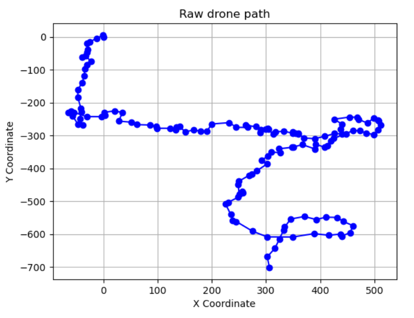
    return lidar_distances

Let's have a look at the raw drone's path based on noisy odometry measurements. Although these measurements contain errors, plotting them can still provide useful insights into the drone's movement.

# Initialize variables to store the current position
x_current = 0
y_current = 0

# Initialize variables to store lists of coordinates
x_coords = [x_current]  # Start at x0 = 0
y_coords = [y_current]  # Start at y0 = 0

# Load lidar data and odometry values from drone_log.jsonl
lidar_data = []
odometry_x = []
odometry_y = []

for step in sensor_data:
    delta_x = step['odometry_x']
    delta_y = step['odometry_y']
    lidar_data.append(step['lidar'])
    odometry_x.append(delta_x)
    odometry_y.append(delta_y)    

    # Update the current position
    x_current += delta_x
    y_current += delta_y
        
    # Append the new coordinates to the lists
    x_coords.append(x_current)
    y_coords.append(y_current)

# Plot the line
plt.plot(x_coords, y_coords, color='blue', linestyle='-', marker='o')
plt.xlabel('X Coordinate')
plt.ylabel('Y Coordinate')
plt.title('Raw drone path')
plt.grid(True)
plt.show()

And here is the output:

Now we know approximately what the path looks like, but we still have no clues. Let's try another approach. In the next code block I convert Lidar measurements from polar to Cartesian coordinates and simulate the drone's movement based on both Lidar data and noisy odometry values. This generates a 3D point cloud of the environment, which I visualize alongside the map data. I do this to gain insights into the approximate area where the drone flew, potentially narrowing down the search area for the drone's starting position.

# Define a function to convert polar coordinates to Cartesian coordinates
def polar_to_cartesian(distance, angle):
    x = distance * math.cos(math.radians(angle))
    y = -1 * distance * math.sin(math.radians(angle))
    return x, y

# Initialize the drone's initial position
approx_start_drone_position = [300.0, 40.0]
drone_positions = []

# Simulate the movement of the drone using lidar data and odometry values
lidar_points = []
for lidar_scan, x, y in zip(lidar_data, odometry_x, odometry_y):
    
    # Update drone position
    approx_start_drone_position[0] += x
    approx_start_drone_position[1] -= y
    
    # Convert lidar data to Cartesian coordinates and update drone position
    for idx, distance in enumerate(lidar_scan):
        angle = idx * 10 % 360  # Calculate angle based on lidar index
        if 0 <= distance <= 200:  # Ensure valid lidar data
            x1, y1 = polar_to_cartesian(distance, angle)
            lidar_points.append([x1 + approx_start_drone_position[0], y1 + approx_start_drone_position[1], 0.0])
            
# Create point cloud from lidar measurements
lidar_pc = o3d.geometry.PointCloud()
lidar_pc.points = o3d.utility.Vector3dVector(lidar_points)
lidar_pc.paint_uniform_color([1, 0, 0])

# Reverse the order of the lines
map_lines_reversed = map_lines[::-1]

# Convert the reversed lines to map data
map_data_rev = [[int(value) for value in line.strip()] for line in map_lines_reversed]

# Convert the map data into a numpy array
map_array = np.array(map_data_rev)

# Convert map data to point cloud
map_points = []
for i in range(map_array.shape[0]):
    for j in range(map_array.shape[1]):
        if map_array[i, j] == 0:  # Free space
            map_points.append([j, i, 0.0])  # Assuming Z coordinate is 0 for the map
                           
# Create point cloud for the map
map_pc = o3d.geometry.PointCloud()
map_pc.points = o3d.utility.Vector3dVector(map_points)

# Visualize the lidar data and the map
o3d.visualization.draw_geometries([lidar_pc, map_pc])

The output is below:

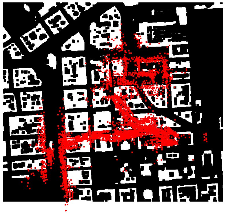
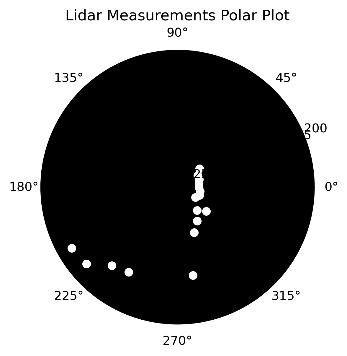
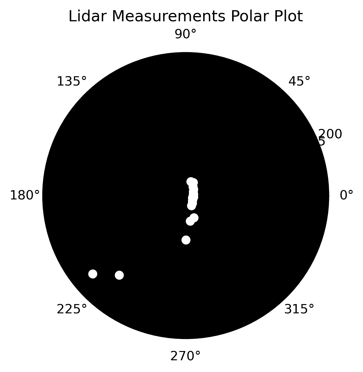
By visualizing the map and the Lidar point cloud together, I can clearly see the drone's path. This allows me to confidently determine that the drone started its journey in the left bottom corner of the map. Now let's create a polar plot to visualize Lidar measurements by plotting valid data points in a circular layout. This helps me see the range and distribution of measurements around the starting point of the drone's path.

def polar_plot(lidar_measurements):
    # Calculate angles for each measurement (in degrees)
    angles_degrees = np.arange(0, 360, 10)  # 36 angles in total
    
    # Filter out invalid measurements
    valid_measurements = [m for m in lidar_measurements if m != -1]
    valid_angles = [angle for angle, m in zip(angles_degrees, lidar_measurements) if m != -1]
    
    # Create the polar plot
    fig = plt.figure(figsize=(4.01, 4.01)) 
    ax = fig.add_subplot(111, polar=True)  # Create a polar subplot
        
    # Plot lidar measurements
    ax.scatter(np.deg2rad(valid_angles), valid_measurements, color='white', marker='o')  # White points
    ax.set_ylim(0, 200)
    ax.set_facecolor('black')  
    ax.grid(False)  
    ax.set_title('Lidar Measurements Polar Plot')
    plt.show()
    
# Polar plot for the start point
start_lidar = sensor_data[0]['lidar']
polar_plot(start_lidar)

And here is the output:

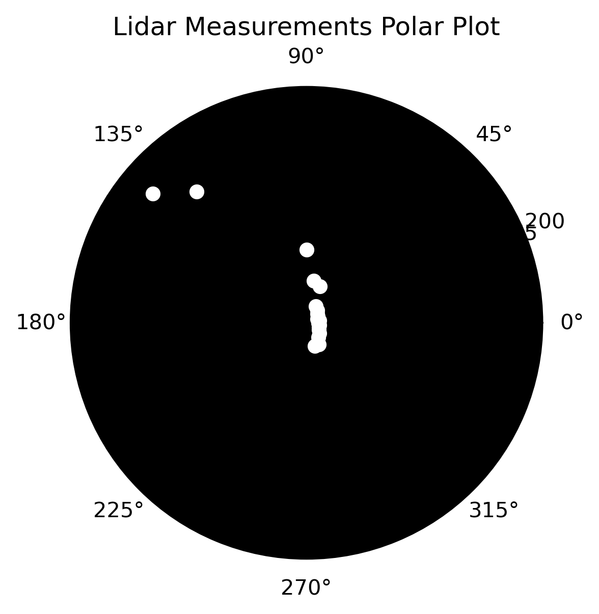
polar plot with input lidar measurements

In the next code, I estimate an approximate starting point for the drone’s path and generate a polar plot of Lidar measurements from that point. This helps verify that the simulated measurements and actual Lidar input data are aligned correctly in terms of angle distribution.

approx_start_drone_position = [300.0, 40.0]
approx_lidar_start = observation_model(approx_start_drone_position[0],approx_start_drone_position[1])
polar_plot(approx_lidar_start)

The output is below:

polar plot with simulated lidar measurements

I noticed that to match the plots correctly, I need to flip the Lidar measurements vertically while ensuring that the 0-degree position remains consistent. I adjust the measurements accordingly and then create a polar plot to verify the alignment:

# Flip lidar vertically
lidar_mes_0 = [approx_lidar_start[0]]
lidar_rest = approx_lidar_start[1:]
lidar_rest = lidar_rest[::-1]
lidar_approx_start_flipped = lidar_mes_0 + lidar_rest
polar_plot(lidar_approx_start_flipped)

Here is the output:

In the next code I define a function to find the position with the minimum error between input Lidar measurements and simulated measurements. The function reverses the order of the simulated measurements (excluding the 0-degree angle) and calculates the error for each position in the specified range. It returns the position with the smallest error, along with the corresponding Lidar measurements.

#Define function for finding point with minimum error in lidar's measurements
def min_error(start_x, end_x, start_y, end_y, lidar_from_input):
    """
    Find the point with the minimum error in calculated lidar's measurements compared to the input lidar measurements.

    Parameters:
    - start_x (int): Starting x-coordinate for the search area.
    - end_x (int): Ending x-coordinate for the search area.
    - start_y (int): Starting y-coordinate for the search area.
    - end_y (int): Ending y-coordinate for the search area.
    - lidar_from_input (list of float): Lidar measurements to compare against.

    Returns:
    - dict: A dictionary with keys 'error', 'x', 'y', and 'lidar_meas'. 
            'error' is the minimum error found, 'x' and 'y' are the coordinates of the best match,
            and 'lidar_meas' contains the lidar measurements at that position.
    """
    min_error_position = {'error': float('inf')}
    for x in range(start_x, end_x):
        for y in range(start_y, end_y):
            if 0 <= x < wi and 0 <= y < he and omap[y,x] == 0:
                
                lidar_meas = observation_model(x, y)
                lidar_mes_angle0 = [lidar_meas[0]]   #leave 0 angle measurement at index 0
                lidar_rest_angles = lidar_meas[1:]   #all measurements but in 0 angle
                lidar_rest_angles = lidar_rest_angles[::-1]
                lidar_measurements = lidar_mes_angle0 + lidar_rest_angles 
                error = np.sum((np.array(lidar_from_input) - np.array(lidar_measurements)) ** 2)
                
                if error < min_error_position['error']:
                    min_error_position['error'] = error
                    min_error_position['x'] = x
                    min_error_position['y'] = y
                    min_error_position['lidar_meas'] = lidar_measurements
                    
    return min_error_position

In the next code I find the real starting and ending points of the drone’s path by comparing the input Lidar measurements with simulated measurements. I search in specific regions of the map where I expect these points to be, but also I have checked the entire map to confirm the results. The function returns and prints the coordinates of the true start and end points.

#check where is the start point of the drone's path
first_lidar = sensor_data[0]['lidar']
result_start = min_error(270, 280, 30 ,40, first_lidar)  
print('First point: ', result_start['x'], result_start['y'])

#check where is the end point of the drone's path
last_lidar = sensor_data[-1]['lidar']
result_last_point = min_error(600, 610, 730 ,740, last_lidar)
print('Last point: ', result_last_point['x'], result_last_point['y'])

The ouput:

First point:  279 36
Last point:  608 737

I define two functions to work with lines on a map. The bresenham_line function generates a list of points forming a straight line between two coordinates using Bresenham's line algorithm. The check_line_on_map function checks which points on the generated line are valid (i.e., not blocked by obstacles) and returns the farthest valid point before hitting an obstacle:

from typing import List, Tuple

def bresenham_line(x0: int, y0: int, x1: int, y1: int) -> List[Tuple[int, int]]:
    """
    Generate a list of points forming a straight line between (x0, y0) and (x1, y1) using Bresenham's algorithm.
    """
    points = []
    dx = abs(x1 - x0) 
    dy = abs(y1 - y0)
    x = x0
    y = y0
    sx = -1 if x0 > x1 else 1  
    sy = -1 if y0 > y1 else 1

    if dx > dy:
        err = dx / 2.0
        while x != x1:
            points.append((x, y))
            err -= dy
            if err < 0:
                y += sy
                err += dx
            x += sx
    else:
        err = dy / 2.0
        while y != y1:
            points.append((x, y))
            err -= dx
            if err < 0:
                x += sx
                err += dy
            y += sy

    points.append((x, y))
    return points

def check_line_on_map(map_data: List[List[int]], line_points: List[Tuple[int, int]]) -> Tuple[int, int]:
    """
    Check which points on the generated line are valid (i.e., not blocked by obstacles) and return the farthest valid point.

    Parameters:
    - map_data (List[List[int]]): 2D list representing the map where 0 indicates free space and non-zero indicates obstacles.
    - line_points (List[Tuple[int, int]]): List of points (x, y) forming the line to check.

    Returns:
    - Tuple[int, int]: The coordinates of the farthest valid point on the line.
    """
    x_right = line_points[0][0]
    y_right = line_points[0][1]
    for point in line_points:
        x, y = point
        
        if map_data[y][x] == 0:
            x_right = x
            y_right = y
        else:
            break  # if it is an object
    return x_right, y_right

In the next code block I start with the initial drone position and Lidar measurements, then iteratively update the drone's path using odometry data while accounting for noise. While short-term noise can be reliable, long-term noise may accumulate and introduce outliers. To address this, I calculate accumulated noise and, if necessary, widen the search area to find the best matching position based on Lidar data. This approach helps ensure accurate tracking of the drone's trajectory despite noisy measurements.

# The start point of the drone's path
x_current = result_start['x']
y_current = result_start['y']
lidar_measurements = result_start['lidar_meas']

x_coords = [x_current]                               # drone's path
y_coords = [y_current]                               # drone's path
st_dev_odometry = 2 * sqrt(NOISE_VARIANCE_ODOMETRY)  #95% of values
cumulative_noise = 0                                 #cumulative error of odometries 


for frame in sensor_data[1:]:
    odometry_x = frame['odometry_x']
    odometry_y = frame['odometry_y']
    odometry_y = -1 * odometry_y
    lidar_data = frame['lidar']
    
    #Make a move
    x_current = x_current + odometry_x
    y_current = y_current + odometry_y

    # take into account noise
    start_x = int(x_current - st_dev_odometry)
    end_x = int(x_current + st_dev_odometry)
    start_y = int(y_current - st_dev_odometry)
    end_y = int(y_current + st_dev_odometry)

    # Check if the drone's path doesn't go through objects:
    line_points = bresenham_line(start_x, start_y, end_x, end_y)
    is_clear = check_line_on_map(omap, line_points)
    end_x = is_clear[0]
    end_y = is_clear[1]
    
    # Find the best suitable point
    current_result = min_error(start_x, end_x, start_y, end_y, lidar_data)
    
    cumulative_noise += st_dev_odometry    #accumulate current noise
    if cumulative_noise > 80:
        cumulative_noise = 80              

    # handle outliers 
    if current_result != {'error': float('inf')}:
        x_current = current_result['x']
        y_current = current_result['y']
    else:
        current_result = min_error(int(start_x - cumulative_noise), int(end_x + cumulative_noise), int(start_y - cumulative_noise), int(end_y + cumulative_noise), lidar_data)
        x_current = current_result['x']
        y_current = current_result['y']
            
    x_coords.append(x_current)
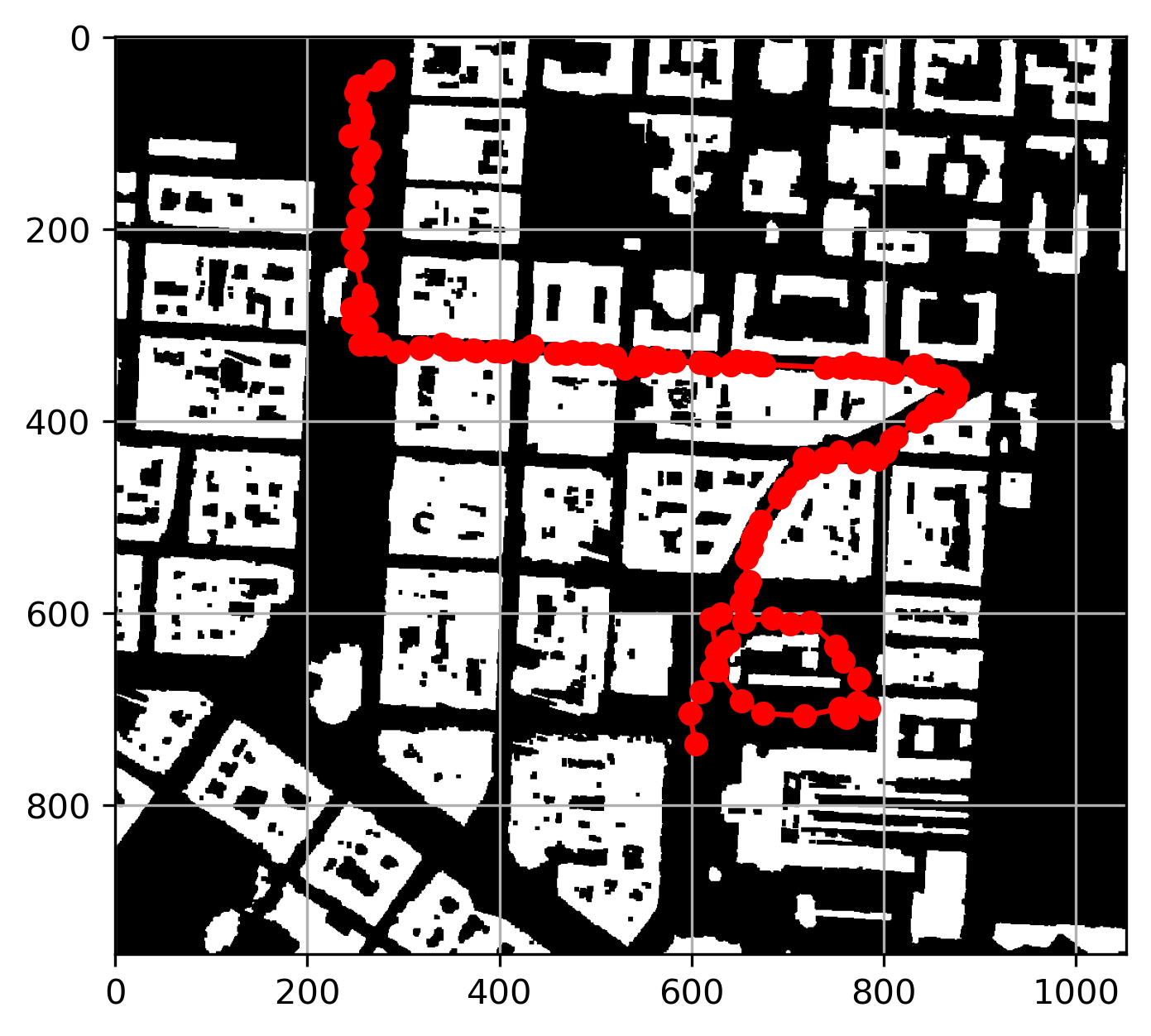
    y_coords.append(y_current)

Here, I visualize the drone's path on the map by overlaying the path coordinates on the map image. The drone's trajectory is plotted in red, allowing for a clear view of its journey overlaid on the city map.

# Visualizing drone path on the map
plt.imshow(omap, cmap='gray')
plt.plot(x_coords, y_coords, marker='o', color='r', linestyle='-')
plt.grid(True)

Here is the plot:

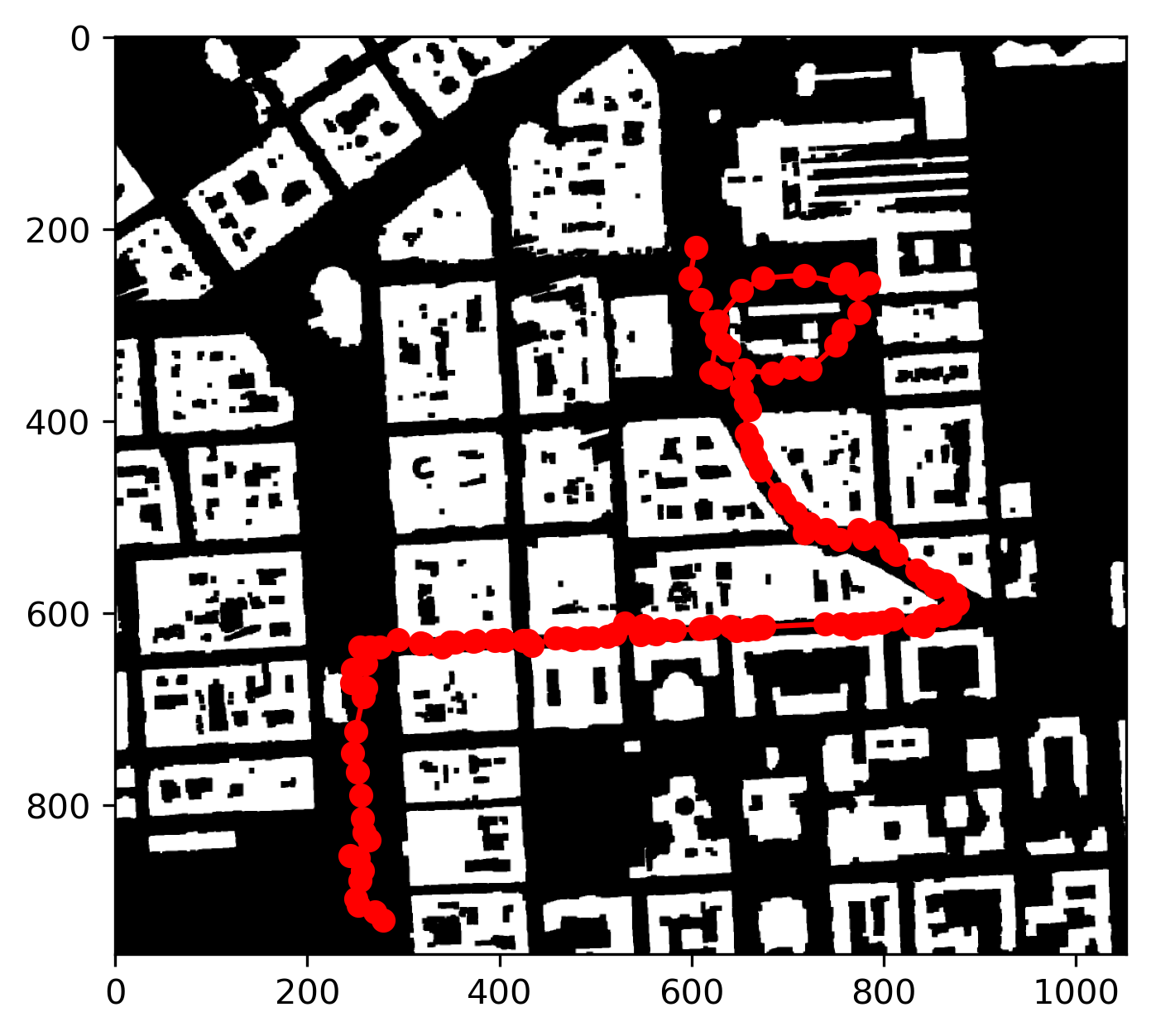
The plotted drone path appears accurate, but further alignment is needed to match it precisely with the PNG map. In the next code, I load the PNG map image and display it using Matplotlib. Since the map plotted from the omap data is vertically flipped compared to the PNG file, we need to flip the drone's path vertically to correctly overlap it with the PNG map. The corrected path is then plotted on top of the PNG map for accurate visualization.

import matplotlib.image as mpimg

# Load and display the image
img = mpimg.imread('map_stadi_bg.png')
plt.imshow(img, cmap='gray', origin='upper')

# Invert y-coordinates to match the coordinate system
y_coords_inv = omap.shape[0] - np.array(y_coords)  # Subtracting from the height of the map

# Plot the drone path
plt.plot(x_coords, y_coords_inv, marker='o', color='r', linestyle='-')
plt.show()

Here is the plot:

This code saves the drone's path coordinates to a CSV file. It writes the x and y coordinates, with appropriate headers, to a file named drone_path.csv. After saving, a confirmation message is printed to indicate the successful creation of the file.

# Specify the file path to save the CSV file
csv_file_path = 'drone_path.csv'

# Write x_coords and y_coords to the CSV file
with open(csv_file_path, 'w', newline='') as csvfile:
    csv_writer = csv.writer(csvfile)
    csv_writer.writerow(['x', 'y'])  # Write header
    for x, y in zip(x_coords, y_coords_inv):
        csv_writer.writerow([x, y])

print(f"CSV file saved successfully at {csv_file_path}")

Conclusion

In this project, I tracked a drone's path through a city using data from its sensors. I combined odometry and Lidar measurements to estimate where the drone flew and visualized its path on a city map and 3D point cloud. By managing sensor noise and adjusting for errors, I ensured the path was accurate. Finally, I saved the drone's path in a CSV file for easy review. This work shows how to use sensor data and maps to track and understand a moving object in a city. The next step for me is to explore Monte Carlo Localization, a method that could further improve the accuracy of the drone's path estimation by using probabilistic techniques.